Chapters
- 1 Getting started
- 2 The interface
- 3 Coordinate systems and conventions
- 4 Modelling
- 5 Materials
- 6 Sections
- 7 Supports, releases and modifiers
- 8 Loads
- 9 Load combinations
- 10 Meshing
- 11 Static analysis
- 12 Dynamic and seismic analysis
- 13 Results
- 14 Design
- 15 Scripting and the AI model builder
- 16 Import and export
- 17 Verification
- 18 Scope and limits
- 19 Troubleshooting
- 20 Glossary and notation
On this page
This chapter describes the static analysis types: linear static, P-Delta, buckling, nonlinear static and pushover, with the frame element and the equation solver they share. For each type it gives the method, its key equations, the options in the Analysis tab and what the results mean. The dynamic and seismic types are in Chapter 12.
11.1 Running an analysis
Analysis > Analysis type lists the twelve analysis types. Pick one, set its parameters and press Run (or Ctrl+Enter).
| Type | Purpose | Chapter |
|---|---|---|
| Linear static | first-order analysis of the load patterns and combinations | 11 |
| P-Delta | second-order analysis: axial loads act on the deflected shape (iterated) | 11 |
| Buckling | elastic critical load factors and buckled shapes for a combination | 11 |
| Nonlinear | geometric and material nonlinearity under load control | 11 |
| Pushover | a lateral pattern increased to a target displacement with plastic hinges | 11 |
| Modal | natural periods, mode shapes and mass participation | 12 |
| Ritz vectors | load-dependent Ritz vectors for the dynamic analyses | 12 |
| Response spectrum | design spectrum by code, modal and directional combination | 12 |
| Equivalent lateral force | base shear and storey forces by code, with accidental eccentricity | 12 |
| Storey checks | torsional irregularity, drift, stability, period, soft storey and mass | 12 |
| Time history | a ground acceleration record integrated in time | 12 |
| Nonlinear time history | direct integration with plastic hinges, gravity first | 12 |
Before the run, the tool checks the model (see the model check) and the inputs the type needs: supports, loads, mass for the dynamic types, a spectrum or a record. If something is missing it says what, in plain words, and nothing is run. The analysis then runs in the background, so the window stays usable; a progress bar shows the steps of the nonlinear and time-history analyses and Cancel stops a long run. Results stay on screen until the next run, and edits to the model do not change them until you run again. The messages of the run (meshing, defaults used, members cut, convergence) are listed under the Run button.
11.2 The frame element and linear static analysis
The linear static analysis solves the equilibrium equations of the whole structure,
where is the global stiffness matrix assembled from the elements, the vector of nodal displacements and the vector of nodal loads, including the equivalent nodal loads of member, area and temperature loads. Each load pattern is solved once and combinations are formed by superposition (9.1).
The frame element is a two-node, twelve-degree-of-freedom element (Przemieniecki) with bending about both axes, axial force, torsion and shear deformation. In the plane of local axes 1 and 2 (bending about axis 3) its stiffness is
for the displacements and rotations , and likewise about axis 2 with and . The axial and torsional terms are and . With a zero shear area, and the element is an Euler-Bernoulli beam. End releases are applied by static condensation, and the element is turned to global axes by the direction cosines of Section 3.2.
Member loads are turned into equivalent nodal loads with the interdependent (Timoshenko) shape functions, so the nodal displacements are exact for any load. The internal forces at the stations are then found by integrating the loads exactly from the end forces, and the deflections by integrating the exact curvature and shear strain, with three-point Gauss rules between load breakpoints and the end displacements fixing the constants. In a static analysis one element per member is therefore exact, and the diagrams need no extra divisions.
Equilibrium check. For every load pattern the run compares the sum of the applied loads with the sum of the reactions, as forces and moments about the origin. The difference is shown in the Results summary ("Sum of the reactions") and should be close to zero; a large difference points to a load on a held degree of freedom or a mechanism. For self-equilibrated patterns such as temperature, it is measured against the size of the reactions.
A fully restrained model (no free degree of freedom) runs in linear static and P-Delta: the displacements are zero, the member forces are the fixed-end forces and the reactions balance them. A fixed-fixed bar heated by gives , for example.
11.3 The equation solver
The stiffness matrix is stored as a sparse symmetric matrix and factorised as
by an up-looking sparse factorisation (Davis 2005). Before factorising, the equations are reordered by the better of reverse Cuthill-McKee and coordinate nested dissection, whichever gives fewer entries in the factor. This keeps a model of 3,000 nodes and 5,500 members to about one second in the browser.
A pivot smaller than of its diagonal term means the structure has no stiffness in some direction: a mechanism, a missing support or end releases that free a joint. The run stops and names the node and the degree of freedom, so the fix is usually a support, a member or a release at that node (Chapter 19).
11.4 P-Delta analysis
The P-Delta analysis includes the effect of the axial forces acting through the displacements. The geometric stiffness , which depends on the axial forces , is added to the elastic stiffness and the solution is iterated:
with the axial forces of each iteration taken from the previous one. The tolerance (default in the Analysis tab) and the largest number of iterations (default 20) are parameters; the run reports the iterations used and whether it converged.
The element geometric stiffness is the consistent matrix of the cubic shape functions. Per unit axial force (tension positive), in the plane of axis 2,
with a torsional term , where is the polar moment of area. Shells contribute a geometric stiffness from their membrane forces.
Because the result depends on the whole load, the P-Delta analysis is run for one combination at a time (chosen in the parameters), not for single patterns. The end forces include the second-order effect of the sway (P-Δ). The moments at stations between the ends are found from those end forces, so the effect of the member's own bow (P-δ) is captured only when slender compression members are divided into several elements (Section 10.1). If the axial load exceeds the elastic buckling load, the iteration has no solution and the run says the structure is unstable under its axial forces.
11.5 Buckling analysis
The buckling analysis finds the load factors by which a base loading must be multiplied for the structure to buckle elastically, with the buckled shapes :
where are the axial forces of a linear analysis under the base loading (a combination or a pattern chosen in the parameters). The eigenproblem is solved in the inverted form with , which allows to be indefinite, by subspace iteration (Bathe). A Sturm sequence count of proves that no factor below the highest one found was missed; when one was, the subspace is enlarged and the solution repeated.
The results list the requested number of buckling factors (default 6) with their shapes. A factor below 1 means the base loading exceeds the elastic critical load; a factor between 1 and about 10 means second-order effects matter and a P-Delta analysis, or the amplification methods of the design code, should be used. The lowest factor of a sway mode is the of EN 1993-1-1 5.2.1 and the elastic buckling load factor of a rational buckling analysis in AS 4100 4.7.2, which AS 4100 uses for the sway amplification factor . When no positive factor exists (for example a base loading in tension only) the run says so.
Divide members into several elements to find member buckling modes between joints; with one element per member only frame (sway) modes are found accurately. When no mesh is set, the buckling analysis divides every member into 4 parts.
11.6 Plastic hinges and fibre elements
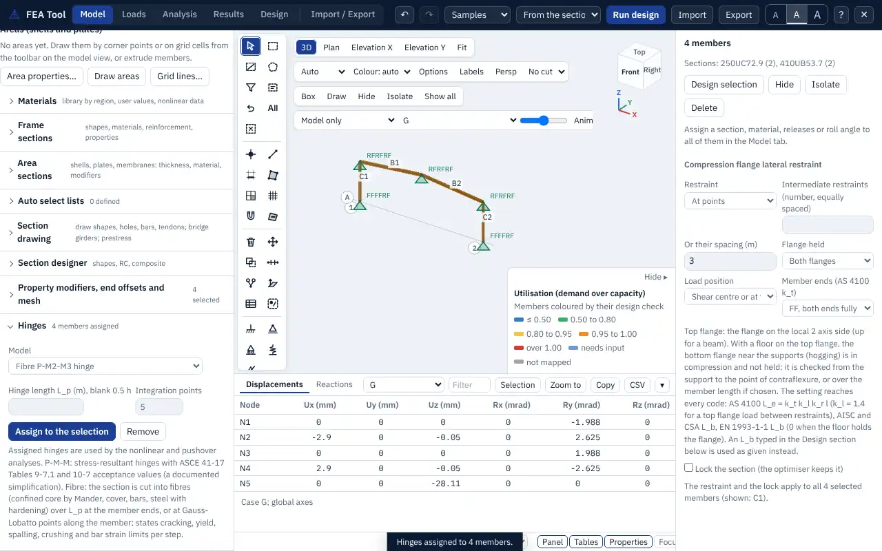
The nonlinear static, pushover and nonlinear time-history analyses model yielding with plastic hinges at the member ends (and at midspan when requested). Model > Hinges assigns them to members:
| Hinge model | Yield surface or method |
|---|---|
| PMM (default) | axial force and both moments interact |
| PM | axial force and the major-axis moment |
| M | moments only |
| Fibre | a force-based fibre element with the section's own materials |
| None | the member stays elastic |
Lumped hinges are rigid-plastic, on a yield surface in the normalised forces , , . For steel I, H and channel sections the surface of Orbison, McGuire and Abel (1982) is used:
For other sections,
and the moment-only hinge uses . Reinforced concrete members use a simplified parabolic P-M surface built from the section and its reinforcement ratio; it is an approximation, and a fibre hinge gives the section's own interaction. The return to the surface is by closest-point projection. A small hardening of times the elastic end stiffness keeps hinges in series unique and raises the plateau by a fraction of a per cent.
Fibre hinges replace the lumped hinge by a force-based fibre element: the section is divided into fibres of its materials (Chapter 5), and the element integrates the section response either at the member ends over a plastic hinge length (default half the section depth) or along the member at 3 to 7 integration points (distributed plasticity). Fibre hinges follow the hysteresis rules of the materials and report the strains of the extreme steel and concrete fibres, so cracking, yield and crushing appear in the results.
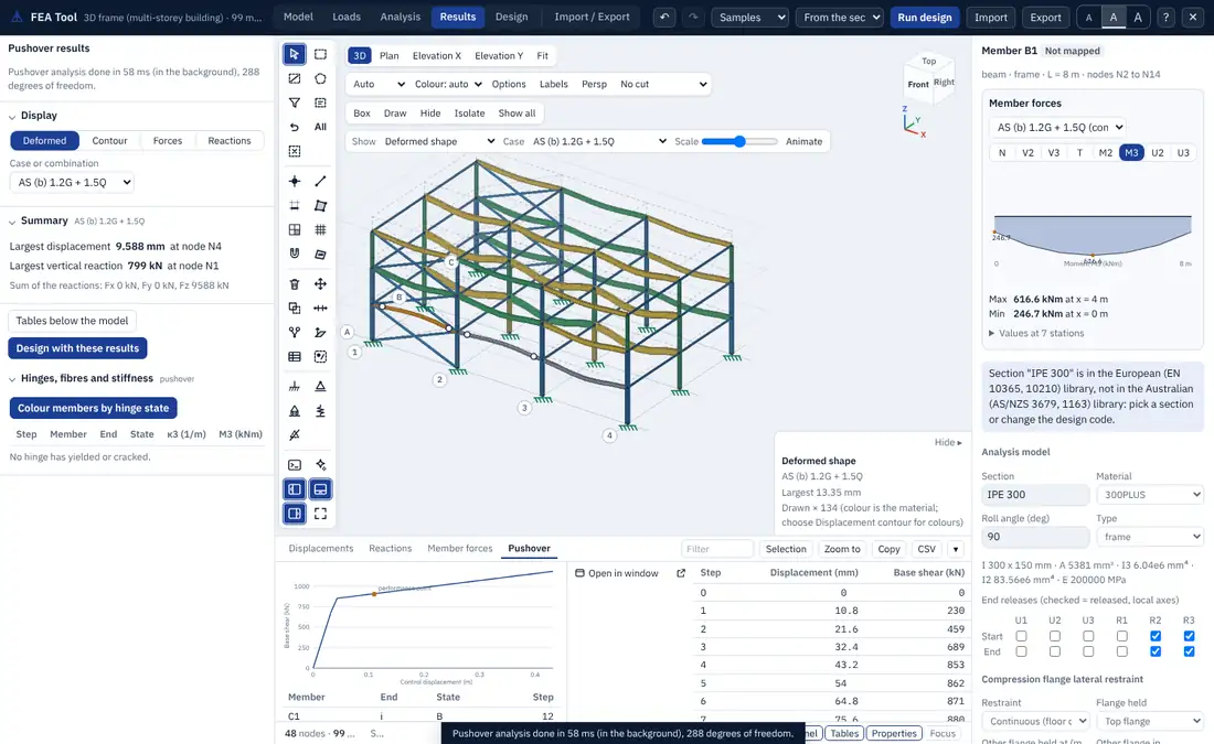
Hinge states. After a nonlinear or pushover run, Results > Hinges, fibres and stiffness lists every hinge that yielded, with its plastic rotation, the ratio to the acceptance limits and the step at which its state changed, and Colour members by hinge state colours the model.
11.7 Nonlinear static analysis
The nonlinear static analysis applies a combination in load steps and finds equilibrium at each step by Newton-Raphson iteration:
where is the load factor of the step, the vector of internal forces and the tangent stiffness. A step that does not converge is halved and tried again. With displacement control, a chosen degree of freedom is driven to a target value instead and the load factor is found from a bordered solution.
Geometry has three options:
- co-rotational large displacement: each element is followed through large rotations; the deformational rotations come from the logarithm of the nodal rotation matrices in the rotated element frame. Use it for cables, arches and large deflections;
- P-Delta: small displacements with the geometric stiffness on the elastic part of each member, and with the plastic hinge rotations taken out of the end rotations, so that a member in a mechanism carries exactly ;
- none: material nonlinearity only.
Cables carry tension only. Member loads keep their direction as the structure deflects. Rigid end offsets are not used, and models with areas cannot be run nonlinearly; the run says so. The parameters are the combination, the number of load steps (default 10), the tolerance and the hinge model.
11.8 Pushover analysis
The pushover analysis applies the gravity load first by load control, then a lateral load pattern by displacement control, increasing it until a control node reaches a target displacement. The defaults use P-Delta geometry and PMM hinges.
| Parameter | Choices |
|---|---|
| Load pattern | modal (proportional to of the first mode in the direction), uniform (proportional to mass) or case (the loads of a pattern, such as a wind pattern) |
| Control node | default the highest node |
| Target displacement | default 4 % of the height of the structure |
| Direction | X or Y |
| Steps | default 40 |
The result is the capacity curve (base shear against the control displacement) with the step at which each hinge formed. Each hinge is given a state on an elastic-perfectly-plastic backbone: B (yielded), IO, LS and CP (the immediate occupancy, life safety and collapse prevention acceptance rotations passed) and C (beyond the end of the plastic plateau). By default the acceptance rotations are taken, in simplified form, from ASCE 41-17 Table 9-7.1 for steel beams (IO, LS and CP at 1, 9 and 11 times the yield rotation , plateau to ) and Table 10-7 for concrete beams (0.010, 0.025 and 0.050 rad). Strength loss after the plateau is not modelled.
Performance point. The target displacement is found by the coefficient method of ASCE 41-17 7.4.3.3.2:
with the effective period from the bilinear idealisation of the curve (7.4.3.2.4),
and the modification factors
where is the elastic period of the first mode, and the elastic and effective stiffness, the spectral acceleration at (g), the yield strength of the bilinear curve, the seismic weight, the effective mass factor (default 1.0), and for site classes A and B, 90 for C and 60 for D to F. when s (and is taken as at least 0.2 s in ), when s, and both are 1 when . is the participation factor times the first mode shape at the control node. The report gives every term with its value and says when lies beyond the end of the curve.