Chapters
- 1 Getting started
- 2 The interface
- 3 Coordinate systems and conventions
- 4 Modelling
- 5 Materials
- 6 Sections
- 7 Supports, releases and modifiers
- 8 Loads
- 9 Load combinations
- 10 Meshing
- 11 Static analysis
- 12 Dynamic and seismic analysis
- 13 Results
- 14 Design
- 15 Scripting and the AI model builder
- 16 Import and export
- 17 Verification
- 18 Scope and limits
- 19 Troubleshooting
- 20 Glossary and notation
On this page
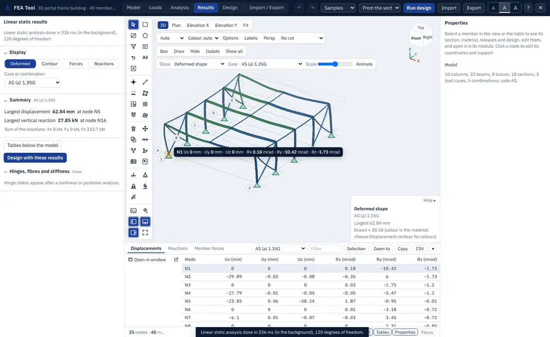
After a run, the Results tab, the model view, the properties panel and the bottom dock all show the results, linked to each other: a value picked in one place is found in the others. This chapter describes the displays (deformed shape, force diagrams, reactions, contours), the legend, the member and node panels, the tables, and the results of the dynamic and nonlinear analyses.
13.1 The Results tab
The Results tab opens with the name of the analysis, its run time, the number of degrees of freedom and whether it ran in the background. Its sections are:
- Display: what the model view shows (Deformed, Contour, Forces with the component N, V2, V3, T, M2 or M3, Reactions), the case or combination, and how values are labelled (Hover, max and min, or Compact labels).
- Summary: the largest displacement and its node, the largest vertical reaction, and the sum of the reactions in X, Y and Z for the case shown, which should balance the applied load.
- Tables below the model opens the bottom dock, and Design with these results goes to the Design tab.
- Sections for the analysis type: modes, buckling factors, hinge states, area results, the slab and wall design, the storey report, the response spectrum base shears, the time history plots and the equivalent lateral forces.
The same choices are on the view toolbar (Show, Case, Scale, Animate), so the results can be changed without the left panel.
13.2 Deformed shape
The deformed shape is drawn from the nodal displacements and, along each member, from the deflections at its stations, so a beam under a distributed load bends as a curve, not as a straight chord. Areas deform with the displacements of their mesh nodes, as a shaded surface or with contour bands on the deformed surface, and frames that share nodes with an area deform with it. The Scale slider sets the magnification; the legend gives the scale used and the largest displacement. Displacement contour colours the members by the size of their displacement.
Envelopes (All strength, TH max, RSA and others) have no single deformed shape, so they are drawn as bands of the maximum and minimum diagrams and listed in the tables.
13.3 Force diagrams and reactions
Forces draws the diagram of one component on every member, in the plane of its local axes: and in the 1-2 plane, and in the 1-3 plane, and in the plane of the member. Values are shown at the maxima and minima and under the pointer, or as compact labels at every peak (key V). The legend gives the case and the largest positive and negative values with the member and position where they occur.
Reactions draws the reaction at every support and spring as force arrows, whose length grows with the magnitude, and moment arcs by the right-hand rule, with the values on hover.
Figure 2.1 shows the diagrams of a frame for one combination, with the member force panel of the selected beam.
13.4 The member force panel
Select a member to see its own diagram in the properties panel: any component (N, V2, V3, T, M2, M3, and the local deflections U2 and U3) for any case or combination, with its largest and smallest values and their positions. Values at n stations opens a table of every component at every station. The stations include both sides of each point load and the ends of the flexible length.
Select a node to see its displacements in every case and combination, in a table that scrolls with the cases.
13.5 Area results and contours
Results > Area results colours the shells, plates and membranes by one result of one case or combination:
| Group | Components |
|---|---|
| membrane forces | , , (kN/m) |
| moments | , , (kNm/m) |
| transverse shears | , (kN/m) |
| stresses at the top and bottom faces | , , , von Mises, principal stresses (MPa) |
| displacement | |
| slab and wall design | required steel top and bottom in directions 1 and 2, shear ratio (Section 14.8) |
The components are in the local axes of each area (Section 3.5). The contour is drawn with 10 to 12 colour bands, each clipped exactly on every triangle of the mesh, so the band edges are true contour lines rather than a blend of corner colours. The legend has a label at every band edge, the minimum and maximum with the node and coordinates where they occur, and the value under the pointer, interpolated within the element. Show mesh draws the element edges; Range from the results fits the bands to the values of the case shown.
The nodal values are averages over the elements of the area meeting at the node. A large jump between neighbouring elements is a sign that the mesh is too coarse there.
13.6 The legend
Whenever colours, bands or diagrams carry values, the legend at the lower right gives the quantity with its display unit, the case, a scale with round numbers (1-2-5 steps), and the largest and smallest values with where they occur. It is drawn at the resolution of the screen, so it stays sharp when the browser zooms. It covers the displacement contours of every case, the force diagrams, reactions, mode and buckling shapes, time history shapes, utilisation colours and the area loads of the Loads tab. Hide folds it away.
13.7 Tables
The bottom dock (Section 2.7) holds the result tables:
| Table | Content |
|---|---|
| Displacements | and of every node (mesh nodes included) for one case |
| Reactions | the six reaction components of every support, spring and area spring |
| Member forces | , , , , , at every station of every member |
| Modes | period, frequency, mass ratios and their sums, mode type |
| Buckling | load factors and their modes |
| Time history | the response history of the recorded nodes |
| Pushover | the capacity curve step by step, and the hinges with their states |
| Nonlinear steps | the load factor, displacement and iterations of each step |
Panels of the Results tab add their own tables to the dock, such as the nodal area results of the slab and wall design.
Every table is sorted by clicking a column heading, filtered by text, limited to the selection with Selection, copied with Copy or saved with CSV, and opened in its own browser window. The values follow the display units. Rows and objects in the model are linked: hovering over a row marks its object, and clicking selects and frames it.
13.8 Results of dynamic and nonlinear analyses
- Modal: choose a mode in Case; Animate plays it, and comma and full stop step through the modes (Figure 12.1).
- Buckling: the buckled shapes, with the factor of each.
- Response spectrum: the cases
RSA,RSA X,RSA Y, the base shear per direction with the scaling factor and its basis, storey shears and the accidental torsion. - Time history: plots of the record, the displacement of the recorded nodes, the base shear and the energy terms against time, with a time slider that drives the deformed shape (Figure 12.2).
- Pushover: the capacity curve with the performance point and its coefficients, and the hinge states at each step (Figure 11.1).
- Nonlinear static and nonlinear time history: the load-displacement history and the hinge states. With fibre hinges, the moment-curvature history of each hinge section and the strains of its extreme fibres are given.
- Equivalent lateral force: the base shear with every term of the code formula and its clause, the storey forces, and a button that adds the storey forces to the model as load patterns.
13.9 Reading the results with care
- Check the sum of the reactions against the applied load for each pattern before reading anything else.
- Compare one or two values with a hand calculation: a beam moment, a column axial force, a first period from .
- Look at the deformed shape of each pattern: a wrong support, a missing connection or a load in the wrong direction is usually obvious.
- For areas, look at the mesh and the contour together, and design from values at the face of supports rather than peaks at point supports.
- Results are those of the model as analysed. Edits made after a run are not reflected until the analysis runs again.