Chapters
- 1 Getting started
- 2 The interface
- 3 Coordinate systems and conventions
- 4 Modelling
- 5 Materials
- 6 Sections
- 7 Supports, releases and modifiers
- 8 Loads
- 9 Load combinations
- 10 Meshing
- 11 Static analysis
- 12 Dynamic and seismic analysis
- 13 Results
- 14 Design
- 15 Scripting and the AI model builder
- 16 Import and export
- 17 Verification
- 18 Scope and limits
- 19 Troubleshooting
- 20 Glossary and notation
On this page
Loads are grouped in load patterns (also called load cases): each pattern is one independent action, such as the dead load, the live load or wind from one direction, with a type that the combination generator uses to apply the factors of the code. This chapter covers the load patterns, self weight, joint, member, area and temperature loads, the joint patterns that describe varying pressures, the mass source of the dynamic analyses and the automatic lateral loads.
8.1 Load patterns
Loads > Load patterns lists the patterns with their name, type, self weight multiplier, automatic lateral load and the number of loads they hold. Add a pattern with a name and a type; the × button deletes one with its loads. Click a row to make it the current pattern for the load forms below.
| Type | Letter | Notes |
|---|---|---|
| dead | G (D) | permanent; usually carries the self weight |
| superdead | G (D) | superimposed dead load; combined with G |
| live | Q (L) | imposed load on floors |
| roof | Q (Lr) | roof live load, with the roof factors of the code |
| snow | S | |
| wind | W | one pattern for each direction; a direction tag (+X, −X, +Y, −Y) is shown in the combination names |
| seismic | E | applied with both signs where the code treats it as reversible |
| temperature | T | |
| fluid | F | liquid pressure |
| earth | H | earth pressure |
| notional | N | notional horizontal forces |
| other | not used by the generator |
Every load is stored in SI (kN, m) whatever the display units, so changing the units never changes a load.
8.2 Self weight
The self weight multiplier of a pattern (1 for the full self weight, 0 for none) adds the weight of every member and area to that pattern. For a member,
per unit length along −Z over the whole length, and for an area per unit area along −Z, with the density of the member's or area's own material and m/s². The weight property modifier scales it. A new, empty model starts with a dead pattern G carrying the full self weight and a live pattern Q.
8.3 Joint loads
Loads > Loads in the current pattern adds a force in kN and a moment in kNm to the selected nodes, in global axes. Negative acts downwards. The list below the form shows the loads of the pattern, each with a × to remove it; Remove loads of the selection clears the loads of the selected objects in the current pattern.
8.4 Member loads
The same panel adds loads to the selected members: a distributed load in kN/m over the whole member, or a point load in kN at a fraction of the length from node . Scripts and imported models can also give partial and trapezoidal loads:
| Kind | Value | Position |
|---|---|---|
distributed (udl) | in kN/m | the whole member, or from to |
point (point) | in kN | at |
trapezoidal (trap) | at to at , in kN/m | from to |
Positions up to 1 are fractions of the member length; larger values are metres from node . A script can ask for metres always.
The direction is one of:
- Global Z, X, Y (
gz,gx,gy): along the global axis, positive in its positive direction; - Gravity (
grav): along −Z, positive downwards; - Local 1, 2, 3 (
l1,l2,l3): along the member's local axes.
A distributed load in a global direction is a load per unit length of the member, not of its projection.
The frame element turns member loads into equivalent nodal loads with the shape functions of the Timoshenko beam, so the displacements at the nodes are exact for any load. The internal forces at the stations are found by integrating the load exactly, so a member need not be divided to get its diagrams right (Section 11.2).
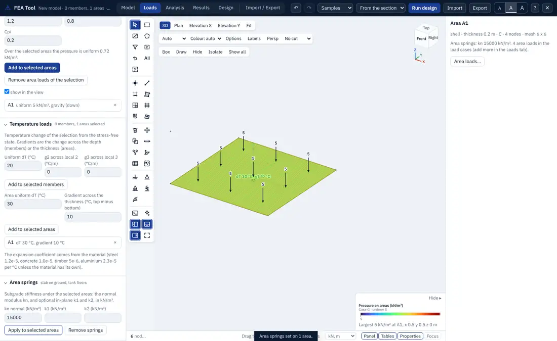
8.5 Area loads
Loads > Area loads adds loads to the selected areas, in kN/m² of the true area of the surface:
- Uniform along a direction: global X, Y or Z, gravity (−Z, positive down), or local 1, 2 or 3.
- Projected: with a global direction, the load is given per unit of projected area, so its value is multiplied by , with the normal of the area and the load direction. Use it for snow or roof live load on a sloping roof, given on plan.
- Pressure on a face: a pressure on the top (+3) or bottom (−3) face of the area, positive when it presses on that face towards the area.
- Pattern: a pressure that varies linearly in space (Section 8.6).
- Hydrostatic and wind: Section 8.7.
The panel shows the resulting pressure as a coloured field on the areas with a legend, and as arrows with values, so the direction and size of each load can be checked before the analysis.
8.6 Joint patterns
A joint pattern describes a pressure that varies linearly in space:
with in kN/m² and , , in metres, in global coordinates or in the local coordinates of each area (measured from its first node along its axes 1, 2 and 3). A clip keeps only one sign:
Define joint patterns in Loads > Joint patterns and use one in an area load of kind pattern with a scale factor. For example, the earth pressure on a wall with lateral pressure coefficient , soil unit weight and ground level is
clipped to the positive part.
8.7 Hydrostatic and wind loads on areas
Hydrostatic. With a fluid of unit weight (9.81 kN/m³ for water) and a free surface at , the pressure at height is
along local 3, with a side factor of +1 or −1 to choose the wetted face. Use it for tank walls and floors.
Wind. With the design wind pressure (kPa) and the external and internal pressure coefficients and ,
along local 3, positive along +3. The coefficients come from the wind standard of the project; the FEA Tool applies them, it does not choose them.
8.8 How area loads reach the nodes
An area load is turned into nodal loads on the mesh by the shape functions of each element:
with exact weights for a constant pressure, 4 × 4 Gauss points on quadrilaterals and 7 points on triangles for a varying one. The mesh therefore carries the load as a consistent nodal load, not by tributary areas. Frames that share nodes with the mesh (Section 10.4) receive load through those nodes.
8.9 Temperature loads
Loads > Temperature loads applies a temperature change to the selected members or areas, measured from the stress-free state.
Members. A uniform change (°C) and gradients , (°C per metre) across the depth along local 2 and local 3. The fixed-end actions are
and the deflected shape includes the free thermal strain and curvature . A positive bends the member towards −local 2. Trusses and cables take only.
Areas. A uniform change gives the membrane strain (not for plates), and a gradient (°C, the +3 face minus the −3 face) gives the curvature
(not for membranes). Area results are the stress resultants of the elastic strain, so an area free to expand reports no forces.
The coefficient comes from the material (Section 5.4). A fully restrained member under a uniform rise gives in compression, which is a useful first check. P-Delta and buckling analyses include the membrane forces of a temperature load, so a restrained plate heated by buckles at the thermal load factor.
8.10 Mass source
The modal, response spectrum, time history and equivalent lateral force analyses need the mass of the structure. Loads > Mass for modal and dynamic analysis sets where it comes from:
- self weight: the mass of every member and area, per unit length and per unit area;
- load patterns, each with a factor: the gravity (−Z) components of the loads of a pattern, divided by , become mass in X, Y and Z:
Typical choices are 1.0 for superimposed dead load and 0.3 for live load; the factors of the seismic code of the project govern.
Node masses (Section 7.8) are added. The mass is consistent by default, or lumped at the nodes when chosen. The rotary inertia of an area is per unit area. Seismic and dynamic setup adds options: mass from patterns in X and Y only, lumping at the diaphragm masters, level masses with their plan size, and an eccentricity of the centre of mass for accidental torsion (Section 12.5).
8.11 Automatic lateral loads
The Auto lateral column of a load pattern links it to the seismic panel or to the wind of the code. A seismic pattern linked this way receives the storey forces of the equivalent lateral force method (Section 12.4) as nodal loads on the model's own joints, which can then be kept as ordinary loads and combined like any other pattern.