Chapters
- 1 Getting started
- 2 The interface
- 3 Coordinate systems and conventions
- 4 Modelling
- 5 Materials
- 6 Sections
- 7 Supports, releases and modifiers
- 8 Loads
- 9 Load combinations
- 10 Meshing
- 11 Static analysis
- 12 Dynamic and seismic analysis
- 13 Results
- 14 Design
- 15 Scripting and the AI model builder
- 16 Import and export
- 17 Verification
- 18 Scope and limits
- 19 Troubleshooting
- 20 Glossary and notation
On this page
This chapter covers the analyses that need the mass of the structure: modal analysis by eigenvectors or Ritz vectors, the equivalent lateral force method, response spectrum analysis, the storey and irregularity checks, and linear and nonlinear time history. It starts with the seismic setup shared by these types and ends with the design spectra and ground motion records.
12.1 Seismic and dynamic setup
Analysis > Seismic and dynamic setup holds the settings shared by the dynamic types. They are saved with the model.
Code and parameters. The seismic code follows the design code, and each has its own parameters:
| Code | Parameters |
|---|---|
| ASCE/SEI 7-22 | , , , , , , , risk category, structural system (for and ) |
| EN 1998-1:2004 | , , ground type A to E, spectrum type 1 or 2, behaviour factor , lower bound factor , drift limit, , structural system |
| NBC 2020 | , , , , , , , , , , importance category, structural system |
| AS 1170.4-2007 | , , site sub-soil class A to E, structural ductility , structural performance factor , structural system (for ) |
The panel plots the design spectrum as you type and lists any input outside the range of the standard, with the clause.
Mass source (Section 8.10), diaphragms (Section 7.9) and levels are set here too. Levels are found from the elevations of the joints, or listed. The accidental eccentricity is given as a ratio of the plan dimension normal to the force; the default is the value of the code (0.05 for ASCE/SEI 7-22 and EN 1998-1, 0.10 for NBC 2020 and AS 1170.4). The default drift limits are also those of the code: for ASCE/SEI 7-22 0.020, 0.020, 0.015 and 0.010 of the storey height for risk categories I to IV; for NBC 2020 0.025, 0.020 and 0.010 for normal, high and post-disaster importance; for EN 1998-1 0.005, 0.0075 or 0.010 of the storey height; and 0.015 for AS 1170.4.
When no mesh is set, the modal, Ritz, response spectrum, time history and equivalent lateral force analyses divide every member into four parts so that the vibration of members between their ends is represented.
12.2 Modal analysis
The modal analysis solves the undamped free-vibration problem
for the lowest modes (12 by default, up to 60), by subspace iteration (Bathe). A Sturm sequence count of at a shift above the last frequency found proves that no mode below it was missed; when one was, the subspace is enlarged and the run repeated. is the consistent mass matrix of the members and areas (or the lumped one when chosen) plus the node masses and the mass from load patterns (Section 8.10).
The mode shapes are normalised so that . For a direction with influence vector (unit ground displacement in that direction), the participation factor, effective modal mass and mass ratio are
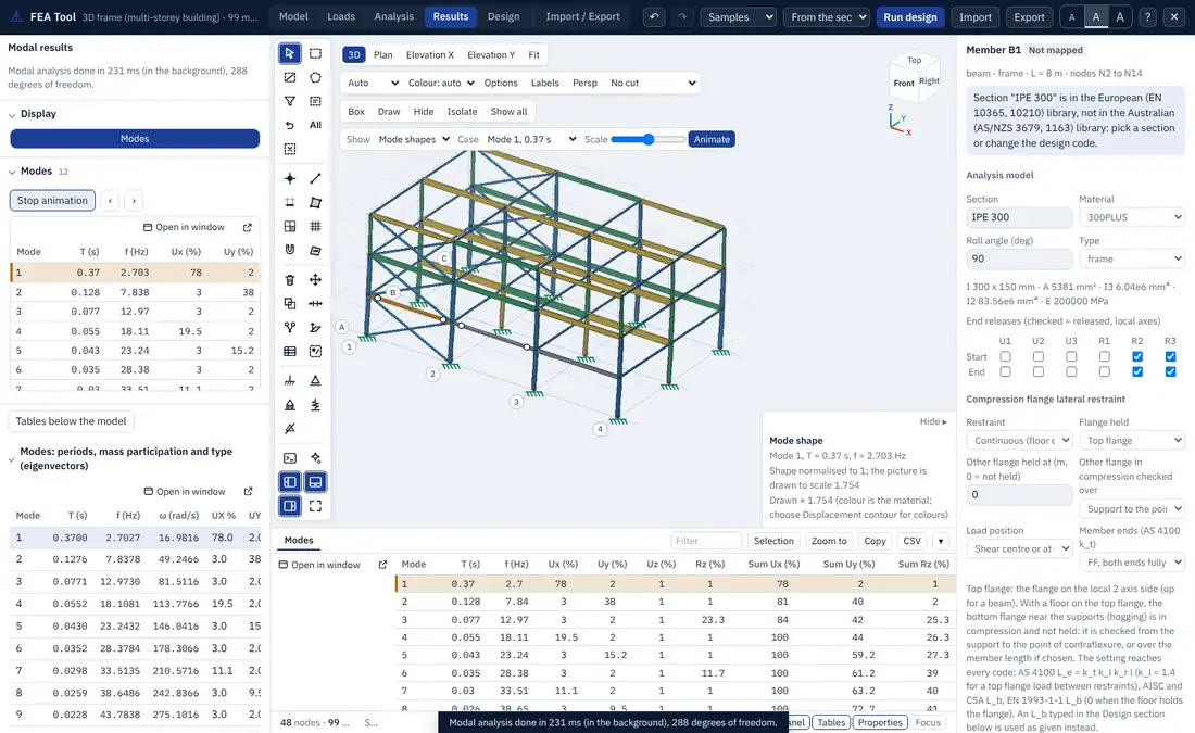
The mode table gives, for each mode, the period, frequency, circular frequency, the mass ratios in UX, UY, UZ and the rotations, their running sums, and the type of the mode. It says how many modes reach 90 % of the mass in each direction, which most seismic codes require.
Mode type. The kinetic energy of each mode is split into the translation of the levels in X and Y, the rotation of each level about its centre of mass, vertical motion and the remainder (local modes of members or slabs). The table names each mode, for example X translation or torsion, so a torsionally sensitive building shows itself in the first modes.
12.3 Ritz vectors
Load-dependent Ritz vectors (Wilson, Yuan and Dickens 1982) are an alternative basis for the dynamic analyses. They start from the static response to a set of loads, by default the acceleration loads in UX, UY and UZ (or chosen load patterns), and build a block Krylov sequence:
with each new block made M-orthonormal to the earlier ones (two Gram-Schmidt passes, vectors below dropped). A small eigenproblem in the Ritz basis, solved by Jacobi rotations, gives the Ritz frequencies and shapes. Because the vectors start from the loads that excite the structure, fewer of them are needed to reach 90 % of the mass than eigenvectors, particularly for structures with many local modes. The run has no Sturm check, and says so.
12.4 Equivalent lateral force
The equivalent lateral force analysis computes the base shear and storey forces of the code, applies them to the levels (at the diaphragm masters, or to the joints of each level in proportion to their mass), and runs a static analysis in each direction with the accidental eccentricity at and (cases ELF X, ELF X+e, ELF X-e and the same for Y). The storey forces can be added to the model as load patterns and combined like any other.
The period is taken from a modal analysis of the model, from the approximate formula of the code, or as typed, within the limits of the code.
ASCE/SEI 7-22 12.8. With the seismic weight ,
and where g. The period is (Table 12.8-2), and a period from the model is limited to (Table 12.8-1). The storey forces are
EN 1998-1 4.3.3.2. with when and the building has more than two storeys, else 1.0, and when the period is approximate. The forces are (Eq. 4.11), or with the first mode shape (Eq. 4.10). When exceeds the report says that 4.3.3.2.1(2) asks for the modal response spectrum method instead.
NBC 2020 4.1.8.11. , not less than the value with ( for walls) and, for , not more than . follows 4.1.8.11.(3) for the structural system, and a period from the model is limited to 1.5 or 2.0 times . The top force is for s, and the rest is distributed in proportion to .
AS 1170.4-2007 Section 6. with , and with , as in (12.5).
12.5 Response spectrum analysis
The response spectrum analysis combines the peak responses of the modes to a design spectrum. For mode and direction , the peak modal displacement is
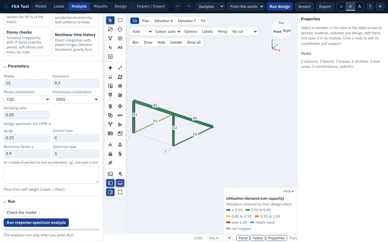
and every other result (member forces, reactions, area forces) follows from it. The modal responses are then combined:
- CQC (default), the complete quadratic combination of Der Kiureghian (1981), which accounts for closely spaced modes:
with and the damping ratio of each mode (0.05 by default, or one value per mode);
- SRSS, , for well-separated modes;
- ABS, the sum of absolute values, an upper bound;
- GMC (Gupta 1990): each mode is split into a rigid part , summed algebraically, and a periodic part , combined by CQC, with between 0 and 1 (default Hz, Hz). Use it where high-frequency modes carry real mass.
The directions are then combined by SRSS or by the 100/30 rule (each direction at 100 % with the others at 30 %, as in EN 1998-1 4.3.3.5.1(3)), or by ABS. The results are cases RSA and RSA X, RSA Y. Because they are magnitudes, a combination that contains them is reported as <name> max and <name> min. A signed option gives each result the sign of the dominant mode, for diagrams that need a sign.
Base shear and scaling. The base shear in each direction is the CQC combination of the modal base shears . With scale to ELF, the forces are scaled up to the equivalent lateral force base shear as the code asks: ASCE/SEI 7-22 12.9.1.4.1 to 100 % of (with the drifts scaled to of Eq. 12.8-6 where it governs, 12.9.1.4.2); NBC 2020 4.1.8.12.(8) to 80 % of , or 100 % for an irregular structure (9), with forces and deflections scaled by (10). EN 1998-1 asks for no scaling, and none is applied for AS 1170.4. The report gives the modal base shear, the target, the factor and its basis.
Storey shears are formed from the modal inertia forces summed above each storey and combined.
Accidental torsion can be applied in two ways:
- static: a storey torsion from the combined storey forces , added to the spectrum results (ASCE/SEI 7-22 12.9.1.5 with 12.8.4.2, EN 1998-1 4.3.3.3.3, NBC 2020 4.1.8.12.(4)(a));
- shifted mass: the modal analysis is run twice in each direction with the centre of mass of every rigid level moved by , and the larger response is kept (NBC 2020 4.1.8.12.(4)(b)).
12.6 Storey checks
The storey checks run the equivalent lateral force and modal analyses and report, for each level and direction, the checks of the code with the clause, the value, the limit, the ratio and the status:
- torsional irregularity: the ratio of the largest to the average drift at the edges of the level, with the extreme points taken at the two edges across the force (ASCE Types 1a and 1b with the amplification ; NBC type 7 from the displacements; EN 1998-1 and );
- storey drift against the limit of the code, with (ASCE) or the factors of the code applied;
- stability coefficient against its limit;
- soft storey, from the storey stiffness against the storey above and the average of the three above;
- mass irregularity from the level masses;
- period against the upper limit of the code.
The level table gives each level's mass, centre of mass, centre of rigidity, polar moment, torsional radius and the eccentricities. The centre of rigidity and the torsional radii come from the flexibility of the level under unit , and at its master:
The weak storey check needs storey strengths and is listed as not covered.
12.7 Time history analysis
The time history analysis integrates the equations of motion under a ground acceleration in one direction:
with relative to the ground. Two families of method are available.
Direct integration. The Newmark method with average acceleration (, , the default) is unconditionally stable and adds no numerical damping. HHT-α () adds controlled damping of the high modes, linear acceleration and Wilson-θ (default ) are also available; linear acceleration, and Wilson-θ below 1.37, are only conditionally stable, so a model with massless degrees of freedom or diaphragm links makes them diverge, and the run refuses them with a plain message. In acceleration form each step solves
with the Rayleigh damping matrix , where for damping ratio at two periods and ()
Damping can also be stiffness-proportional, mass-proportional or none.
Modal superposition. The response is the sum of the modal responses, each integrated with the piecewise-exact recurrence for a linearly varying load (Chopra 5.2), with a damping ratio per mode. It is fast and exact for a piecewise linear record, but limited to the modes computed.
Energy check. The run tracks the input energy, kinetic energy, strain energy and damping energy,
and reports the balance error , which is zero to round-off for average acceleration. A large error points to a time step that is too long.
Initial state. A load case or combination can be applied statically first, so that the dynamic response starts from the gravity state. Otherwise static loads are not included, and the time history results are combined with static cases as needed.
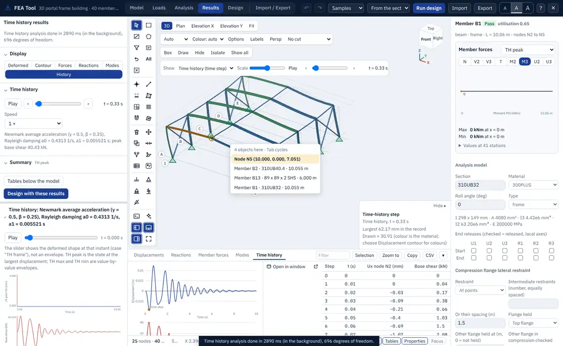
Results. The run gives the displacement history of the recorded nodes, the member force history of the recorded members, the base shear history, storey drifts, the energy history, and three result cases: TH peak (the state at the largest displacement, with member results), and the envelopes TH max and TH min. When the number of nodes times the number of steps is at most 200,000, the history of every node is kept and the deformed shape can be drawn at any time step: the time slider and Animate play it, and the comma and full stop keys step through it. The time step, duration, output interval and sub-steps are parameters; at most 20,000 steps are accepted.
12.8 Nonlinear time history
The nonlinear time history adds plastic hinges (PMM, M or none, Section 11.6) and, optionally, P-Delta geometry to the direct integration. At each step Newton iterations solve
with the accelerations and velocities from the Newmark average-acceleration relations and from the initial stiffness. Gravity is applied first. The plastic work appears in the strain term of the energy balance. The results add the hinge states with their plastic rotations and the ratio to the acceptance limits, and a case THNL end with the state at the end of the record. Models with areas cannot be run nonlinearly.
12.9 Design spectra and ground motions
Code spectra. The spectrum of each code is built from the parameters of the seismic setup, in g:
- ASCE/SEI 7-22 11.4.5.2 (two-period): for , up to , up to and beyond, with and , divided by for the response spectrum method (12.9.1.2). A multi-period table (11.4.5.1) can be pasted instead.
- EN 1998-1 3.2.2.5 (design spectrum, Eqs. 3.13 to 3.16) with , , , of Table 3.2 or 3.3 for the ground type and spectrum type, , the behaviour factor and the lower bound ; the elastic spectrum of 3.2.2.2 when :
- NBC 2020 4.1.8.4.(6): interpolated between the given values, with the larger of and for s and beyond 10 s; times for the response spectrum method (4.1.8.12).
- AS 1170.4-2007 6.4: with the spectral shape factor of Table 6.4 for the site sub-soil class (modal values for s), and the design value .
Your own spectra and records. Analysis > Your own spectra and records accepts a response spectrum as two columns (period in s and in g, m/s² or mm/s², or frequency instead of period) and a ground motion as time and acceleration pairs or as one column at a given time step, pasted from a spreadsheet or a CSV file. The parser plots the data, sorts or resamples where needed, and lists what it did: unequal time steps resampled, a record that does not start at zero, duplicate periods, negative values. Saved spectra and records are kept in the model file and can be picked in the response spectrum options and as the ground motion of a time history. PEER NGA .AT2 files are read directly.
Synthetic records. Sine, half-sine pulse, frequency sweep and step records can be generated for checks. A spectrum-compatible synthetic record can be generated from a target spectrum (duration, time step, rise and strong-motion phases), adjusted iteratively until its response spectrum matches the target; the panel reports the mean misfit. No recorded earthquake is supplied with the tool.
Scaling records. A suite of records can be scaled to a target spectrum over a period range around , as ASCE/SEI 7-22 16.2 or EN 1998-1 3.2.3.1.2(4) ask. The response spectrum of each record is computed by the piecewise-exact single-degree-of-freedom solution (with the maximum-direction value for a pair of components), and the report gives the scale factors, the mean spectrum, its ratio to the target and whether the suite passes.